Solving The Kuramoto-Sivashinsky Equation Using FFT
The Kuramoto-Sivashinsky equation is solved by taking the derivatives in Fourier space.
The Kuramoto-Sivashinsky equation is a simple 1-dimensional model of instabilities in flames \[\begin{equation} \frac{\partial u}{\partial t} = - \frac{\partial^2 u}{\partial x^2} - \frac{\partial^4 u}{\partial x^4} - u \frac{\partial u}{\partial x} \ , \end{equation}\]
or succintly, \[\begin{equation} u_t = - u_{xx} - u_{xxxx} - u u_x \end{equation}\]
To solve this partial differential equation, first, we need to take the spatial domain to Fourier domain. To do that we need the Fourier transform. The derivatives we have above can be calculated as follows using the property of Fourier transform \[\begin{aligned} \frac{d}{dx}u(x, t) & \overset{FT}{\leftrightarrow}i\kappa\cdot \hat{u}(\kappa, t) \ , \\ \frac{d^2}{dx^2}u(x, t) & \overset{FT}{\leftrightarrow}-\kappa^2 \cdot \hat{u}(\kappa, t) \ , \\ \frac{d^4}{dx^4}u(x, t)& \overset{FT}{\leftrightarrow} \kappa^4 \cdot \hat{u}(\kappa, t) \ , \end{aligned}\]
where \(\hat{u}(\kappa, t)\) lives in the Fourier domain. Now, if we go back to the spatial domain by inverse Fourier transform, we have successfully calculated the derivatives. The rest is integrating the resulting equation. For that we will use solve_ivp function from scipy.integrate using the LSODA solver. The code below does all this and plots the result.
import numpy as np
import matplotlib.pyplot as plt
from scipy.integrate import solve_ivp


def kuramoto_sivashinsky(t, u, kappa, nu):
    uhat = np.fft.fft(u)
    d_uhat = 1j*kappa*uhat      # first derivative
    d2_uhat = -kappa**2*uhat    # second derivative
    d4_uhat = kappa**4*uhat # forth derivative
    d_u = np.fft.ifft(d_uhat)
    d2_u = np.fft.ifft(d2_uhat)
    d4_u = np.fft.ifft(d4_uhat)
    du_dt = -u*d_u - d2_u - nu*d4_u
    return [du_dt.real]


nu = 1   # diffusion coeff.
L = 64   # length
N = 256  # num of points
dx = L/N
x = np.arange(-L/2, L/2, dx)  # space domain

kappa = 2*np.pi*np.fft.fftfreq(N, d=dx)  # discrete wavenumbers

# initial condition
u0 = np.cos((6 * np.pi * x) / L) + 0.5 * np.sin((2 * np.pi * x) / L)

# time domain
dt = 0.5
t = np.arange(0, 400*dt, dt)

sol = solve_ivp(kuramoto_sivashinsky, t_span=[t[0], t[-1]], y0=u0,
              method="LSODA", t_eval=t, args=(kappa, nu))
u = sol.y.T

# plot the result
xx, tt = np.meshgrid(x, t)
plt.figure(figsize=(5,5))
plt.contourf(xx, tt, u, levels=100, cmap=cm.jet)
plt.xlabel(r"$x$")
plt.ylabel(r"$t$")
plt.colorbar()
plt.tight_layout()
plt.show()
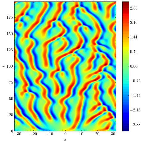
One thing to note is that using the Fourier method automatically imposed periodic boundary conditions.